Shubik Auction II
Note to the Teacher:Here we have a sequential game with randomness.
A theoretical analysis without reference to the game tree
is not possible, therefore we refer to the Excel sheet
ShubikAuction.xls here.
The three players version is only briefly discussed in the text, but the analysis
is done in the secret Excel sheet
ShubikAuction3.xls. This should remain secret since
the three player version is a very good (although rather tedious and difficult) student project.
Another option for a project would be to provide the Excel sheet and let the students
produce, collect, display, and interpret the data.
Finally, Section 4 is still work in progress.
Prerequisites: Chapters
1,
3,
4,
5,
and 6.
This is a continuation of Shubik Auction I.
Remember that there, knowing the maximum number of moves in advance leads to the
slightly disappointing solution
that the player who will eventually not have the last move will not even start bidding, when
playing optimally.
But what happens if the number of possible bidding rounds is finite but unknown in advance?
Or if then number of rounds is finite, but after every move the game could randomly end?
This chapter is mainly an exercise for simultaneou games with randomness,
but it also discusses already the connection to games with nonperfect information, and even
the connection to games with incomplete information.
1. Possible Sudden End
What happens if we don't know in advance which player has the last move?
Assume that there is still a maximum number of rounds, but the game could terminate after
each round with a given fixed probability p.
This makes the game fairer, more profitable for the auctioneer, and also much more interesting.
SHUBIK AUCTION(A,B,n,p):
Two players, Adam and Bob, bid sequentially for an item, with bids increasing by increments of 10 dollars.
The item has a value of A for Ann and a value of B for Beth.
The game ends if one player passes, i.e. fails to increase the bid,
or after the maximum bidding round n has been reached.
But there is a third way how the game could end:
after every bid, the game may also terminate randomly with probability p.
After the game ends, both players pay their highest bids, but only the one
with the higher (most recent) one gets the item.
Of course, for p=0 we just get the non-random version discussed above.
How does the backwards induction analysis change?
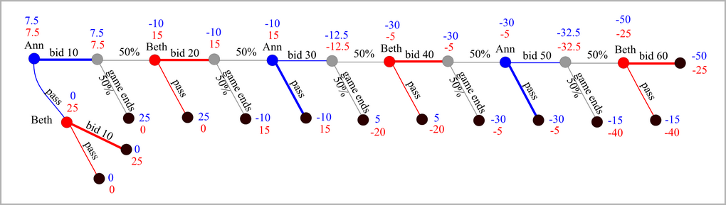
Let us look at a concrete example SHUBIK AUCTION(35,35,6,0.5).
The game tree is shown below, already with expected payoffs for the positions and
recommended moves obtained from backward induction analysis filled in.
In Beth's last position, she will bid 60. That implies that the expectations at this position
for Ann and Beth are -50 and -25. Therefore the expectations at the last random position
are the averages of (-50,25) and (-15,-40), namely (-32.5,-32.5).
Since -30 is larger than -32.5, Ann passes instead of bidding 50.
Proceeding this way, we get expected payoffs of 7.5 for both players
at the beginning of the game.
Note also that Ann plays slightly different than in the case without the possibility of a random ending.
Like there, she will usually not bid, with the one exception of her very first move.
What might be the reason for this change? Well, there is a large possibility that the
game ends right after this first bid, and Ann gets the item, and bidding is still cheap at
this very beginning.
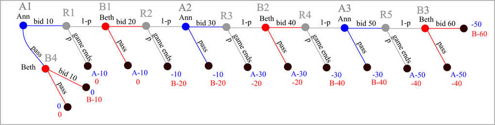
Is it possible to try the analysis not only for concrete parameters,
but once and for all for arbitrary parameters A, B, and p?
Of course, for fixed n=6, the structure of the game tree remains the same,
and the payoffs can be expressed in terms of A and B, as shown below.
Ann's positions are labeled as A1, A2, A3, Beth's positions as B1, B2, B3, and B4,
and the random move positions as R1, R2, ... .
- In position B3, Beth faces payoffs of B-60 versus -40, so she will bid 60 provided
B-60 > -40, i.e. B > 20.
- The expected payoffs for Ann and Beth when facing the random position R5 are
(1-p)(-50) + p(A-50) = pA-50 for Ann and
(1-p)(B-60) + p(-40) = (1-p)B+20p-60 for Beth if B > 20.
If B ≤ 20, they are A-50 and -40.
- Next is position A3. If B > 20, Ann faces an expected payoff of pA-50
and a payoff of -30. The first number is larger for A > 20/p, therefore Ann will bid then.
If B ≤ 20, Ann bids for A > 20.
Therefore, Ann's and Beth's expected payoffs in position A3 are
- pA-50 and (1-p)B+20p-60 if B > 20 and A > 20/p,
- -30 and B-40 if B > 20 and A < 20/p,
- A-50 and -40 if B ≤ 20 and A > 20,
- -30 and B-40 if B ≤ 20 and A < 20,
In case B > 20 and A=20/p we get a tie, and it is not totally clear what
Beth's expected payoff would be in that case. So we omit this singular case, as well as
the case B ≤ 20 and A = 20.
- The second and fourth case could be combined.
Thus, the expected payoffs in position R4 for Ann and Beth are
- (1-p)(pA-50) - 30p and (1-p)((1-p)B+20p-60)+p(B-40) if B > 20 and A > 20/p,
- -30(1-p)) -30p and (1-p)(B-40)+p(B-40) if either (B > 20 and A < 20/p) or (B ≤ 20 and A < 20),
- (1-p)(A-50) -30p and -40(1-p)+p(B-40) if B ≤ 20 and A > 20.
Are you still with me? But you probably see that this analysis can be done, for arbitrary
parameters. Unfortunately the number of cases increases at each one of Ann's and Beth's positions.
Instead of pursuing this further, let us take a different approach here,
making numerical computations for different values A, B, n, p, and collecting the results in
tables. For this, we use the Excel sheet
ShubikAuction.xls.
There are different sheets, for different maximum number n of rounds.
On each sheet you can input A, B, and p, then the expected payoffs for Ann and Beth
in the different positions are displayed below each vertex.
Pressing "Ctrl-h" starts a macro creating a table and chart of Ann's and Beth's expected payoffs
at the beginning of the game for p varying from 0 to 1.
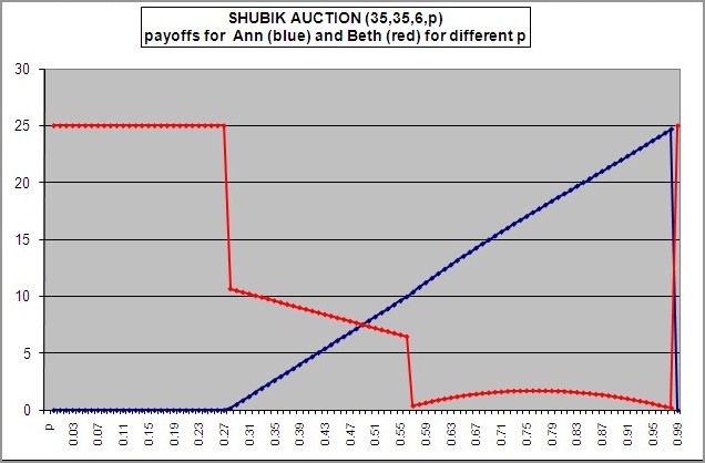
For instance, select the 6-rounds sheet and input A=35 and B=35.
We get the chart below to the left. Obviously the lines jump at some values of p.
In our example, these are around p=0.28 and around p=0.57.
These are the values where Ann's or Beth's optimal strategies change.
For p between 0 and 0.28 Ann will always pass and Beth always raise the bid.
For p between 0.28 and 0.57 we get the same pattern as above for p=0.5: Ann bids 10, but
doesn't try higher bids, whereas Beth always bids. For larger p, both will always
bid. The probability for a sudden end is just high enough making daring a bid worthwhile.
Note that Ann's strategy changes around p=0.28 and around p=0.57, but it is Beth's payoff that
dramatically changes at these values.

If Ann values the item more, let's say A=45, Ann will obviously try harder to get the item.
We get the chart above to the right, which now has 4 strategy patterns.
For p between 0.45 and 0.55, Ann always bids, whereas Beth would pass on her 20 bid
(while still prepared to bid 40 and 60, but of course, these positions will not be reached then).
This strange behavior has to do with Ann bidding for smaller p, due to the higher
worth of the item for Ann, whereas this middle level p is not promising enough payoff
for Beth, given the relatively low worth of the item for Beth.
2. Imperfect and Incomplete Information
Let us play a different variant now, a variant where Nature, instead
of deciding after every move whether the game should be terminated, makes
this decision when to terminate the game at the beginning of the game, but doesn't tell
this decision to Ann and Beth. So we have a maximum number of n moves,
and the game starts with a random move deciding the actual number of moves that
will be played. Further assume that with probability p1 this number will
equal 1, with probability p2 this number will
equal 2, and so on. Obviously this probabilities must add up to 1,
p1+p2+...+pn=1.
Since this random move about the actual number of moves played is not revealed to Ann
and Beth, this game is a simultaneous game with randomness and imperfect information.
On the other hand, it is rather obvious that for appropriate parameters
p1,p2,...,pn this new game is just our SHUBIK AUCTION(A,B,n,p).
Since the probability that SHUBIK AUCTION(A,B,n,p) ends after the first round is p,
that it ends after the second move is p2, and so on, we have to select
p1=p, p2=p2, ..., pn-1=pn-1,
and pn=pn-1. Below is the extensive form of the game equivalent to
SHUBIK AUCTION(35,35,6,0.5).

We can even describe this new, more interesting game as a game of incomplete information.
We play at most n rounds, but it could be less. Note that incomplete information
means that the extensive form is not fully known to the players.
However, in games of incomplete information players need "beliefs" about the
structure of the game---without such beliefs, players would not be able to make
any decisions. If we assume that both players have the same beliefs about how likely
the length of the game is 1, 2, ... n moves, then we arrives exactly at the
game of imperfect information discussed above. Only in case of different beliefs,
we could not model the game in this way.
3. Three Players (optional)
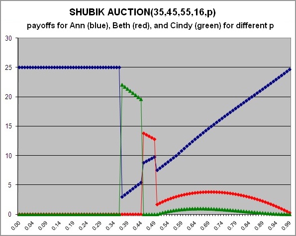
SHUBIK AUCTION(A,B,C,n,p):
Three players, Ann, Beth, and Cindy, bid sequentially in cyclical order for an item
worth A dollars for Ann, B dollars for Beth, and C dollars for Cindy.
After every round the game may end randomly with probability p.
Again this game can be analyzed using an Excel sheet.
The different payoffs for optimal play for a fixed example and variable probability p
are shown below. Again, the probabilities where one or more of the players change
their strategies are rather visible from the graph.
4. The Auctioneer enters the game (optional)
Assume we are playing the 2 player variant, SHUBIK AUCTION(A,B,n,p),
but before the start,
the Auctioneer has one move: Deciding the probability p. Furthermore assume that the item
is worthless for the auctioneer, so the payoff for him or her is just the total amount of
money paid. We arrive at another sequential 3-player game, which we call
SHUBIK AUCTION w.A.(A,B,n) where the auctioneer has the first move and only this one move.
How would the auctioneer decide p, and how much payoff could he or she expect?
Exercise: What would happen in the game SHUBIK AUCTION w.A.(A,B,n) if the item
would be worth 30 dollars to the auctioneer?
Of course, again it depends on the parameters A, B, and probably to a lesser extend on n.
But note that p is no longer a parameter of the game, it is chosen within the game.
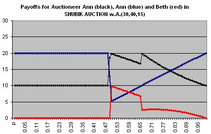
As can be seen from this chart, the Auctioneer should choose p slightly larger than 1/2
or slightly larger than 2/3 to obtain an expected payoff of almost 20 dollars.
References
- Martin Shubik, The Dollar Auction Game: A Paradox in Noncooperative
Behavior and Escalation, The Journal of Conflict Resolution, 15, (1971) 109-111.
- Dollar Auctions, a Wikipedia article at
http://en.wikipedia.org/wiki/Dollar_auction.
Exercises
- Below is the graph of SHUBIK AUCTION (45,35,14,p). Are the payoffs identical
to SHUBIK AUCTION(43,35,6,p)? Explain.

...........
- Find the precise values p for SHUBIK AUCTION(35,35,6,p) where Ann's or Beth's payoffs "jump".
Do the same for SHUBIK AUCTION(45,35,6,p) and SHUBIK AUCTION(45,35,14,p)
...
- Can you explain why, when increasing the probability slowly and at some point of p
Ann's strategy changes, Ann's payoff remains about the same but Beth's payoffs jumps?
...
-
Consider the version of the imperfect information variant discussed in Section 2,
where there is a random and secret decision before the game starts
whether to end after 1, 2, ... 7 rounds, and where each one of these
options has equal probability 1/7. Formulate the game as a game with
perfect information, where after the first round the game ends with probability
p1, after the second round with another probability
p2, and so on. How large are p1, p2, ... .
...
Project: Consider the version of the imperfect information variant discussed in Section 2,
where there is a random and secret decision before the game starts
whether to end after 1, 2, ... n rounds, and where each one of these
options has equal probability 1/n. The game can also be formulated as a game with
perfect information, where after the first round the game ends with probability
p1, after the second round with another probability
p2, and so on. How large are p1, p2, ... , depending on n?
Modify the Excel sheet ShubikAuction.xls such that these games, for various maximum game length can be modelled.
Explore a few cases.
...
Project: Consider SHUBIK AUCTION(A,B,14,p), where 20 ≤ A ≤ B. Will Beth ever pass?
...
Project: As discussed above, SHUBIK AUCTION(45,35,6,p) has four strategy patterns.
Can you find parameters A, B, n, and p where there are 5 or more different strategy patterns?
...
- .....
...
- .....
...
- .....
...